Paper Reading Notes

Categories: Turbulence 2024-04-01

Notes

Concept

1. Boundary Layer

The troposphere extends from the ground up to an average altitude of 11km, but often only the lowest couple kilometers are directly modified by the underlying surface. We can define the boundary layer as that part of the troposphere that is directly influenced by the presence of the earth’s surface, and responds to surface forcings with a timescale of about an hour or less. These forcings include frictional drag, evaporation and transpiration, heat transfer, pollutant emission, and terrain induced flow modification. The boundary layer thickness is quite variable in time and space, ranging from hundreds of meters to a few kilometers.

Boundary layer (also known as the planetary boundary layer, PBL, or the atmospheric boundary layer, ABL)

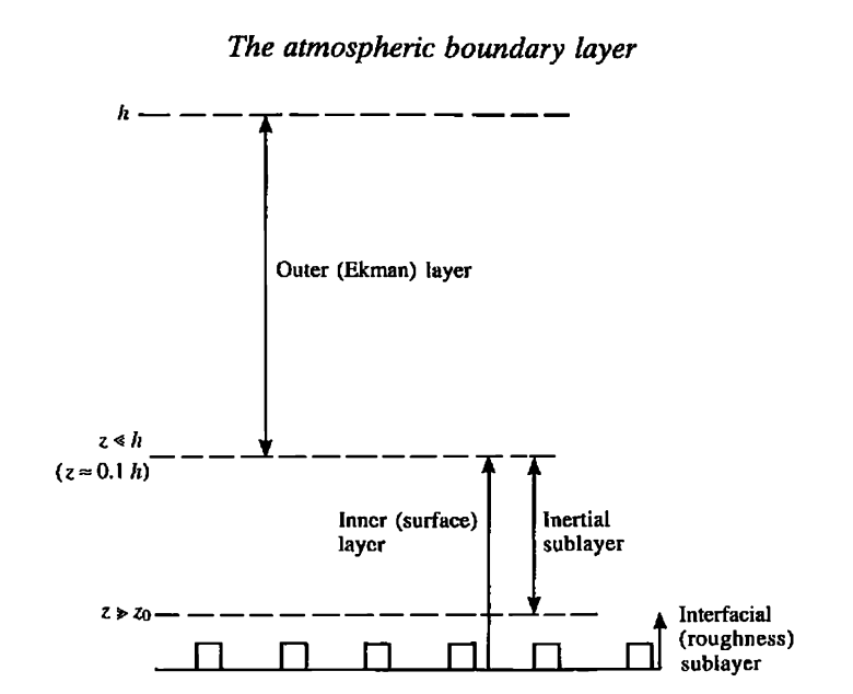
2. Inertial Sublayer(ISL)

3. Roughness Sublayer(RSL)

How to define the RSL and ISL in atmospheric boundary layer flow? The atmospheric boundary layer (ABL) is the part of the troposphere that is directly influenced by the presence of the earth’s surface and responds to surface forcings, such as heat, moisture, and momentum transfers, over a timescale of an hour or less. Within the ABL, the Roughness Sublayer (RSL) and the Inertial Sublayer (ISL) are two important concepts that help in understanding the distribution and transfer of scalars (e.g., temperature, moisture) and momentum near the surface.

Roughness Sublayer (RSL)

The Roughness Sublayer is the portion of the atmospheric boundary layer immediately above the ground surface, extending upwards to a few heights of the roughness elements (such as trees, buildings, or other surface features). The depth of the RSL depends on the nature and distribution of the surface roughness. The RSL is characterized by:

• High levels of turbulence caused by the mechanical breakup of the airflow over and around the roughness elements.
• Non-logarithmic velocity profiles, unlike in the layers above, due to the direct influence of the roughness elements on the flow.
• Enhanced scalar gradients (such as temperature and humidity) due to the close proximity to sources and sinks at the surface.

Inertial Sublayer (ISL)

The Inertial Sublayer lies above the RSL and extends up to the lower portion of the surface layer, which itself is part of the larger atmospheric boundary layer. The ISL is characterized by:

• A relatively uniform flow where the effects of the surface roughness are less pronounced, and the flow is primarily influenced by the earth’s rotation and the resulting geostrophic winds.
• Logarithmic velocity profiles, indicative of a turbulent, but more homogeneous flow than in the RSL.
• Reduced direct influence from the surface roughness, allowing for the application of Monin-Obukhov similarity theory, which describes the profiles of wind speed, temperature, and moisture using dimensionless stability parameters.

Defining RSL and ISL

The exact height and characteristics of the RSL and ISL can vary significantly depending on local surface roughness, atmospheric stability (which itself is influenced by surface heating or cooling), and the presence of obstacles or features that affect the flow. Generally, the RSL is considered to extend from the surface to roughly 1 to 2 times the height of the roughness elements, while the ISL is found directly above the RSL and extends to the point where the effects of surface roughness become negligible, and the flow characteristics are more influenced by the larger-scale atmospheric motions.

In practical applications, defining the exact boundaries of the RSL and ISL requires empirical data and modeling, as these layers are dynamic and respond to changing atmospheric conditions. Researchers and practitioners use various measurement techniques, including towers equipped with anemometers and thermometers, lidar, and sodar, to study these layers and their interactions with the surface.

How to get the RSL and ISL height by a wind profile? Determining the heights of the Roughness Sublayer (RSL) and the Inertial Sublayer (ISL) from a wind profile involves analyzing the vertical distribution of wind speeds within the Atmospheric Boundary Layer (ABL). These analyses often require field measurements collected from meteorological towers, lidar, or sodar systems equipped with anemometers at various heights. Here’s a general approach to estimate the RSL and ISL heights from wind profile data:

1. Collect and Prepare Wind Profile Data

Wind speed measurements should be collected at multiple heights above the ground. The more levels of measurement available, the more detailed the profile analysis will be. Ensure the data are averaged over a suitable period (e.g., 10 to 30 minutes) to filter out short-term fluctuations and highlight the underlying profile characteristics.

2. Analyze the Logarithmic Wind Profile

The wind profile in the ISL (and part of the surface layer above it) can often be represented by a logarithmic relationship between wind speed ((U)) and height ((z)):

[ $U(z) = \frac{u_*}{\kappa} \ln \left( \frac{z - d}{z_0} \right) $]

where:

• ($U(z)$) is the wind speed at height ($z$),
• ($u_*$) is the friction velocity,
• ($\kappa$) is the von Kármán constant (approximately 0.4),
• ($d$) is the displacement height, often relevant in environments with considerable canopy or obstacle height,
• ($z_0$) is the roughness length.

Plotting wind speed against the logarithm of height and fitting this equation allows for identification of the logarithmic layer, primarily associated with the ISL. The best fit to this logarithmic profile helps to identify where the profile begins to deviate from the logarithmic behavior, usually marking the transition from the ISL to the RSL or canopy layer below.

3. Identify the RSL and ISL Heights

• RSL Height: Below the height where the logarithmic wind profile begins, deviations due to the influence of surface roughness elements (e.g., buildings, vegetation) become noticeable. The layer between the ground and where the logarithmic fit becomes appropriate is considered the RSL. The upper boundary of the RSL is somewhat subjective but is generally identified where the wind profile starts to follow the logarithmic relationship closely.

• ISL Height: The ISL is characterized by the range over which the logarithmic wind profile equation provides a good fit to the observed wind speeds. The upper boundary of the ISL is less distinctly defined but transitions into the surface layer, where the effects of atmospheric stability become significant, and the Monin-Obukhov similarity theory applies.

4. Considerations for Stability and Roughness

• Atmospheric Stability: The stability of the atmosphere (neutral, stable, or unstable) affects the wind profile shape. Corrections for stability can be applied using Monin-Obukhov similarity theory, particularly for heights above the ISL.
• Surface Roughness: The value of the roughness length (($z_0$)) and displacement height (($d$)) are crucial for accurately determining the wind profile and, by extension, the heights of the RSL and ISL. These values are often estimated based on the surface characteristics or through more sophisticated modeling techniques.

This process involves a combination of empirical data analysis and theoretical modeling. Advanced techniques, including numerical modeling and the use of specialized instrumentation (like sonic anemometers for turbulence measurements), may provide more precise insights into the characteristics of the RSL and ISL within the ABL.

Matlab code to do the fitting to identify the ISL. To identify the Inertial Sublayer (ISL) by fitting a logarithmic wind profile to wind speed data collected at various heights, you can use MATLAB’s curve fitting tools. The logarithmic wind profile equation, which is often valid within the ISL, is given by:

[ $U(z) = \frac{u_*}{\kappa} \ln\left(\frac{z - d}{z_0}\right) $]

where:

• ($U(z)$) is the wind speed at height (z),
• ($u_*$) is the friction velocity,
• ($\kappa$) is the von Kármán constant (approximately 0.4),
• ($d$) is the displacement height (often 0 for simplicity in basic applications),
• ($z_0$) is the roughness length.

For this example, I’ll simplify the equation by assuming ($d = 0$) and treating ( $\frac{u_*}{\kappa}$ ) and ($z_0$) as fitting parameters. Here’s a MATLAB script that fits the logarithmic profile to the data and plots the results:

1
2
3
4
5
6
7
8
9
10
11
12
13
14
15
16
17
18
19
20
21
22
23
24
25
26
27
28
29
30
31
32
33
34
35
36
% Example wind speed data (m/s) at various heights (m)
z = [2, 4, 10, 20, 40]; % Heights above ground
U = [1.2, 1.8, 2.5, 3.0, 3.8]; % Wind speeds

% Ensure variables are column vectors
z = z(:);
U = U(:);

% Define the logarithmic wind profile function
% Assuming d = 0 for simplicity
logWindProfile = @(b, z) (b(1) .* log(z ./ b(2)));

% Initial guesses for [u_*/kappa, z_0]
initialGuess = [0.1, 0.1]; % These are rough guesses and may need adjustment

% Curve fitting
[beta, R, ~, CovB] = nlinfit(z, U, logWindProfile, initialGuess);

% Calculate fitted wind speeds
U_fit = logWindProfile(beta, z);

% Plotting
figure;
scatter(z, U, 'filled');
hold on;
plot(z, U_fit, '-r');
xlabel('Height above ground (m)');
ylabel('Wind Speed (m/s)');
legend('Measured Wind Speed', 'Fitted Logarithmic Profile', 'Location', 'best');
title('Wind Profile Fitting');
grid on;

% Display fitting parameters
fprintf('Fitted Parameters:\n');
fprintf('u_*/kappa: %f\n', beta(1));
fprintf('z_0 (roughness length): %f m\n', beta(2));

This script does the following:

1. Defines example wind speed data at various heights.
2. Assumes ($d=0$) and fits the logarithmic wind profile to the data.
3. Uses nlinfit for nonlinear curve fitting, which requires the Statistics and Machine Learning Toolbox.
4. Plots the measured wind speeds and the fitted logarithmic profile for visual comparison.
5. Prints the fitted parameters, which include a combined term for friction velocity and von Kármán constant, and the roughness length.

Make sure to replace the example $z$ and $U$ variables with your actual measurements. The initial guesses for the fitting parameters might need adjustment based on your specific data set. If the starting point of wind profile is not $z = 0$, how to do the fitting? If the starting point of your wind profile data is not at ($z = 0$), which is common in practical measurements due to instrument limitations or obstacles, you can still fit the logarithmic wind profile to your data by adjusting the model slightly. The key adjustment involves ensuring your fitting function accounts for the actual range of heights where your measurements start. The logarithmic wind profile remains the same, but you’ll be fitting it to data that starts from a minimum height ($z_{\text{min}}$) rather than from ground level.

Here’s how you can modify the MATLAB code to handle such cases:

1
2
3
4
5
6
7
8
9
10
11
12
13
14
15
16
17
18
19
20
21
22
23
24
25
26
27
28
29
30
31
32
33
34
35
36
% Example wind speed data (m/s) at various heights (m), starting above z=0
z = [10, 20, 30, 40, 50]; % Heights above ground in meters
U = [2.3, 3.2, 3.8, 4.1, 4.5]; % Corresponding wind speeds in m/s

% Ensure variables are column vectors
z = z(:);
U = U(:);

% Define the logarithmic wind profile function accounting for z starting above 0
logWindProfile = @(b, z) (b(1) .* log((z - b(3)) ./ b(2)));

% Initial guesses for [u_*/kappa, z_0, d]
initialGuess = [0.1, 0.1, 0]; % These are rough guesses and may need adjustment

% Curve fitting
[beta, R, ~, CovB] = nlinfit(z, U, logWindProfile, initialGuess);

% Calculate fitted wind speeds
U_fit = logWindProfile(beta, z);

% Plotting
figure;
scatter(z, U, 'filled');
hold on;
plot(z, U_fit, '-r');
xlabel('Height above ground (m)');
ylabel('Wind Speed (m/s)');
legend('Measured Wind Speed', 'Fitted Logarithmic Profile', 'Location', 'best');
title('Wind Profile Fitting');
grid on;

% Display fitting parameters
fprintf('Fitted Parameters:\n');
fprintf('u_*/kappa: %f\n', beta(1));
fprintf('z_0 (roughness length): %f m\n', beta(2));
fprintf('Displacement height (d): %f m\n', beta(3));

In this adjusted script, the fitting function logWindProfile now includes an additional parameter (b(3)), which represents the displacement height (d). This parameter can compensate for the data starting above the ground. Note that in practical ABL studies, (d) is often significant in environments with tall roughness elements like forests or urban areas, where it represents the height below which wind speeds are significantly reduced due to obstructions.

In this context, adding (d) as a fitting parameter allows you to effectively shift the baseline of your logarithmic profile to match the starting point of your measurements. This can improve the fit if your data indeed start from a height where the wind profile is already influenced by surface roughness or other factors.

Remember, the quality of the fit and the interpretation of (d) will depend on the characteristics of your measurement site and the height range of your data. It’s also crucial to have a good initial guess for the parameters to ensure the fitting process converges to a meaningful solution.

How to determine the displacement height d? is it equal to the distance from ground to the starting point? The displacement height ((d)) in the context of atmospheric boundary layer (ABL) studies is not simply the distance from the ground to the starting point of your wind profile measurements. Instead, it has a specific physical meaning and is determined through empirical or theoretical methods. The displacement height is particularly important in environments with tall roughness elements, such as forests or urban areas, and represents the height above the ground at which the wind speed theoretically reduces to zero due to the drag induced by these roughness elements. It effectively shifts the zero plane of the wind profile upwards, accounting for the bulk effect of obstacles on the airflow.

Determining Displacement Height $d$

There are several methods to estimate (d), depending on the available data and the specific characteristics of the study area:

1. Empirical Relations

For certain types of terrain or vegetation, empirical relations based on measurements have been developed to estimate (d). For example, (d) is often estimated as a fraction of the vegetation height ($h_v$) for forests or crops:

[ $d \approx \frac{2}{3} h_v$ ]

This ratio can vary depending on the type of vegetation or surface roughness.

2. Direct Measurement

In urban environments or areas with well-defined obstacles, (d) can sometimes be estimated by direct observation and measurement of the effective height of the obstacles. This approach requires a detailed understanding of the area’s geometry and the distribution of roughness elements.

3. Profile Fitting

When detailed wind profile data are available, ($d$) can be estimated by fitting a theoretical wind profile (such as the logarithmic wind profile) to the measured data. This involves treating ($d$) as a fitting parameter alongside the roughness length ($z_0$) and the friction velocity ($u_*$). The fitting process adjusts ($d$) to match the observed profile, subject to the constraints of the theoretical model.

4. Numerical Modeling

Advanced numerical models that simulate the $ABL$ and its interaction with surface roughness can also be used to estimate ($d$). These models require detailed inputs about the surface characteristics but can provide spatially and temporally resolved estimates of ($d$) and other boundary layer parameters.

Is (d) Equal to the Starting Height of Measurements?

No, ($d$) is not inherently equal to the height at which your measurements start. Instead, it’s a theoretical concept that describes how much the presence of surface roughness “displaces” the apparent origin of the wind profile above the actual ground level. The starting height of your wind speed measurements is determined by practical considerations (such as the minimum height at which instruments can be mounted), while ($d$) is a parameter that needs to be estimated based on the characteristics of the surface and the wind profile itself.

In summary, determining the displacement height (($d$)) requires an understanding of the surface conditions and often involves empirical estimates, direct measurements, profile fitting, or numerical modeling, rather than being directly equated to the height at which wind speed measurements commence.

Starting with Initial Estimates

1. Initial Guesses: You often start with initial guesses for (d), ($z_0$), and ($u_*$) based on empirical knowledge, literature values for similar environments, or simple assumptions (e.g., (d) as a fraction of the height of roughness elements).

2. Fitting the Model: You then fit the wind profile model to your data with these initial parameters. Modern fitting algorithms can adjust these parameters iteratively to minimize the difference between the measured wind speeds and the model.

3. Refining Estimates: The fitting process provides refined estimates of ($d$), ($z_0$), and ($u_*$). This step may reveal the need to adjust the model or the fitting parameters, leading to additional iterations.

Breaking the Loop

• Physical Reasoning: The physical significance of ($d$) and ($z_0$) helps break what might seem like a loop. ($d$) represents the effective shift of the wind profile’s origin due to obstacles, while ($z_0$) characterizes the surface’s aerodynamic roughness. Both have physical interpretations that guide their initial estimates.

• Iterative Refinement: The iterative process of fitting and refining the parameters allows for convergence on a set of values that best represent the actual wind profile. It’s not so much a loop as it is a convergence process.

• Independent Methods: For certain environments, ($d$) can be estimated independently (e.g., a fraction of canopy height in forests) and then used as a fixed parameter in fitting, reducing the number of variables that need to be iteratively adjusted.

Practical Approach

In practice, if the landscape or the height of roughness elements (like trees or buildings) is fairly uniform, initial estimates of (d) can be made based on empirical relationships or direct measurements, reducing the dependency loop. The fitting process then fine-tunes these estimates based on how well they match the observed wind profile.

Conclusion

The iterative nature of estimating ($d$) through profile fitting does not constitute an endless loop but rather a convergent process guided by physical principles, empirical knowledge, and mathematical optimization techniques. By carefully selecting initial guesses and iteratively refining them, it’s possible to accurately model the wind profile and estimate key parameters, including the displacement height.

full code without d, and the starting point of the wind profile is not the ground level, under which to do the fitting and confirm the RSL and ISL. To create a MATLAB script that fits a wind profile to measured data without prior knowledge of the displacement height ($d$) and when measurements do not start at ground level, we’ll assume ($d$) and the roughness length (($z_0$)) are unknowns to be estimated. This script will use the logarithmic wind profile equation, allowing ($d$) and ($z_0$) to be fitting parameters alongside a scale factor that essentially represents ($\frac{u_}{\kappa}$), where ($u_$) is the friction velocity and ($\kappa$) is the von Kármán constant.

The script will perform the following steps:

1. Define the measured wind speeds and corresponding heights.
2. Fit the logarithmic wind profile to this data, estimating ($d$), ($z_0$), and the scale factor.
3. Plot the measured data and the fitted profile for comparison.

Here is the MATLAB code:

1
2
3
4
5
6
7
8
9
10
11
12
13
14
15
16
17
18
19
20
21
22
23
24
25
26
27
28
29
30
31
32
33
34
35
36
37
38
39
40
41
% Required for using nlinfit if Statistics and Machine Learning Toolbox is available
if ~exist('nlinfit', 'file')
    error('This script requires the Statistics and Machine Learning Toolbox.');
end

% Example wind speed data (m/s) at various heights (m), not starting from z=0
z = [10, 20, 30, 40, 50]'; % Heights above ground (ensure column vector)
U = [2.3, 3.2, 3.8, 4.1, 4.5]'; % Wind speeds (ensure column vector)

% Logarithmic wind profile function including displacement height (d) and roughness length (z0)
logWindProfile = @(b, z) b(1) .* log((z - b(3)) ./ b(2));

% Initial guesses for [scale factor, z_0, d]
% Note: These should be based on the expected conditions but are generally unknown.
% Here, we provide a reasonable starting point for the optimization.
initialGuess = [0.1, 1, 5]; % [Scale factor, z0, d]

% Nonlinear curve fitting
opts = statset('nlinfit');
opts.RobustWgtFun = 'bisquare';
[beta, ~, R, ~, ~] = nlinfit(z, U, logWindProfile, initialGuess, opts);

% Generate a smooth curve for the fitted profile over the observed height range
z_fit = linspace(min(z), max(z), 100)';
U_fit = logWindProfile(beta, z_fit);

% Plotting the results
figure;
plot(U, z, 'bo', 'MarkerFaceColor', 'b'); hold on; % Measured data
plot(U_fit, z_fit, 'r-', 'LineWidth', 2); % Fitted profile
xlabel('Wind Speed (m/s)');
ylabel('Height (m)');
title('Wind Profile Fitting');
legend('Measured Data', 'Fitted Logarithmic Profile', 'Location', 'Southeast');
grid on;

% Display the estimated parameters
fprintf('Estimated Parameters:\n');
fprintf('Scale factor (u_*/kappa): %.3f\n', beta(1));
fprintf('Roughness length (z0): %.3f m\n', beta(2));
fprintf('Displacement height (d): %.3f m\n', beta(3));

Points to Note:

• Initial Guesses: The success of the fitting procedure depends significantly on the initial guesses for the scale factor, ($z_0$), and ($d$). You may need to adjust these based on your specific scenario.

• Statistical Toolbox Requirement: The nlinfit function used for nonlinear regression requires MATLAB’s Statistics and Machine Learning Toolbox.

• Plot Interpretation: The plotted results will show the measured wind speeds at their respective heights and the fitted logarithmic wind profile. This visual comparison can help confirm the appropriateness of the fitted model and the estimated parameters, including the displacement height, which aids in identifying the RSL and ISL.

This script provides a basic framework for fitting a logarithmic wind profile to measured data when starting above ground level and without prior knowledge of the displacement height. Adjustments may be necessary to better suit specific data sets or environmental conditions.

4. Mixing Layer

5. Drag Coefficient

Data Process

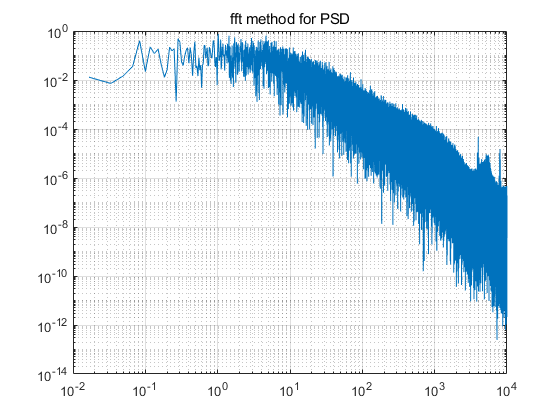
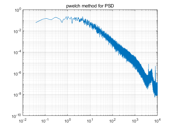
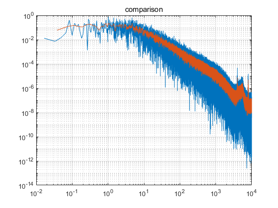
1. Spectrum

Difference between fft and pwelch in Matlab. The following code can give the correct amplitude.

1
2
3
4
5
6
7
8
9
10
11
12
13
14
15
16
17
18
19
20
21
22
23
24
25
26
27
28
clear all
format long

fs = 20000;
N = 1200000;  %data length
t = (0:N-1)/fs; 
rawData = importdata('F:\LiFei\Data\Hotwire\Nanshan20240127\Data\y-50mm\x_0mm\20240202_x0000.0_y-050.0_z0065.0.out');
data =rawData.data;
u = data(1:1200000,4);
flu = u-mean(u);

p_fft = fft(flu,N);
psd_fft = 2*abs(p_fft(1:end/2+1)).^2/fs/N;  %power spectra density is energy density/t，energy spectra is the absolute of the fft result. Due two the symmetry of fft, need to multiply 2 to calculate all the power.  The frequency of the first point is 0 Hz, which is not symmetrical.
freq = linspace(0,fs/2,length(psd_fft));
[pxx,f] = pwelch(flu,[],[],[],20000); % The second parameter denotes the windows, we may use hamming(N) windows here to reduce the data.
figure;
plot(freq, psd_fft);
set(gca, 'xscale', 'log');
set(gca, 'yscale', 'log');
title('fft methods for PSD');
grid on
hold on
% figure;
plot(f, pxx);
set(gca, 'xscale','log');
set(gca, 'yscale','log');
title('pwelch method for PSD');
grid on

2. Amplitude modulation

Single-point

Two-point

Predictive model

3. Statistical Properties

Figure

1.concept related to the large-scale and small-scale.

1. From Blackman ¹

Papers

1. The role of coherent structures in subfilter-scale dissipation of turbulence measured in the atmospheric surface layer

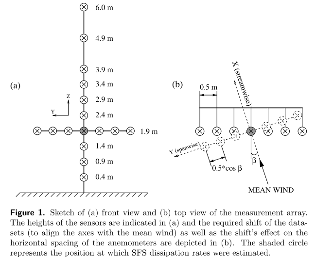
Field Measurement, 16 sonic anemometers, 6m high, 3m wide,

LES subfilter-scale (SFS),

Field measurement

sampling frequency 20Hz. The original data were separated into 30-min periods and individual subsets were selected based on the level of stationarity of wind direction, wind speed and turbulent statistics.

Obukhov length: \(L=\frac{-u_{*}^{3}\left< \theta \right>}{\kappa g\left< u_3'\theta ' \right>}\) *z/L =+0.10 (weakly stable conditions, top panel)*

*z/L = −2.39 (unstable conditions, bottom panel).*

The use of Taylor’s hypothesis has been well accepted for data measured in the atmospheric surface layer with turbulence intensities up to 30% and more

[Wyngaard J C and Clifford S F 1977 Taylor’s hypothesis and high-frequency turbulence spectra]

Velocity gradient calculation:

The gradients of the filtered velocity and temperature were computed along all three axial directions at the location where the vertical and horizontal arrays intersect. This was done using a centered finite-differencing scheme with the filtered data from the nearest sensors for the spanwise and vertical gradients, and the filtered data from the time series at half the filter scale (invoking Taylor’s hypothesis) for the streamwise gradients.

Two point correlation \(R\left( r \right) =\left< u\left( y,t \right) u\left( y+h,t \right) \right> /\left( \sigma _{u\left( y,t \right)}{\sigma _u}_{\left( y+h,t \right)} \right)\)

By finding the lag of the maximum correlation between each pair, a linear relation can be found (by least-squares fit) between the measurement height and the lag associated with the maximum correlation. The arctangent of the slope yields a characteristic inclination angle along which the maximum correlations occur.

2. Packet structure of surface eddies in the atmospheric boundary layer

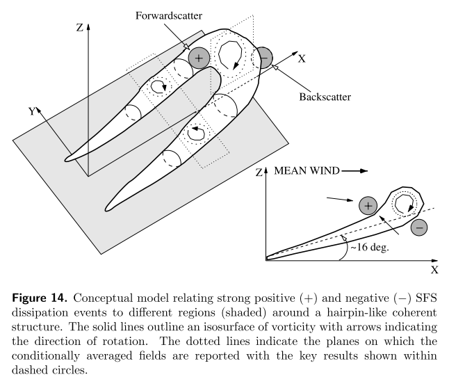
They reveal large-scale ramp-like structures with downstream inclination of 3◦–35◦. This inclination is interpreted as the hairpin packet growth angle following the hairpin vortex packet model of Adrian, Meinhart, and Tomkins.

Hairpin vortex

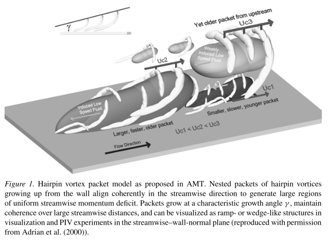
This model provides a possible basis for numerous structural features of wall turbulence including very-long, low-speed streaks, multiple uniform streamwise momentum zones, and the presence of large-scale structures throughout the entire boundary layer.

The hairpin vortex packets form a hierarchy of dynamically similar structures whose size increases in proportion to their distance above the wall, at least through the region of the logarithmic layer. But, to observe many levels of this hierarchy, it is necessary to have a very large separation between the outer scale of the boundary layer, i.e., its thickness, and the inner scale, i.e., the viscous length scale, at which the smallest vortices are formed. This scale separation increases with Reynolds number.

3.Observations of coherent turbulence structures in the near-neutral atmospheric boundary layer

4. Turbulent energy scale budget equations in a fully developed channel flow

Kolmogorov’s equation can be derived from the Navier–Stokes equations, using homogeneity and isotropy: \(-\left< \left( \Delta u_1 \right) ^3 \right> +6\nu \frac{d}{dr}\left< \left( \Delta u_1 \right) ^2 \right> =\frac{4}{5}\left< \epsilon \right> r\) with the increment $\Delta u_1\left( r \right) \equiv u_1\left( x_1+r \right) -u_1\left( x_1 \right) $, where $u_1$ is the longitudinal (streamwise) velocity component, This equation indicates that the mean energy transferred at a scale $r$ is made up of both the energy lost through the turbulent advection ($-\left< \left( \Delta u_1 \right) ^3 \right>$) and the energy lost by molecular destruction ($6\nu \frac{d}{dr}\left< \left( \Delta u_1 \right) ^2 \right>$). It can be interpreted as an energy budget equation involving $\left< \epsilon \right>$, but it can also be thought of as an equation which provides information about $\left< \epsilon \right>$. The equation is a relatively simple means of obtaining $\left< \epsilon \right>$, as the second- and third-order moments can be inferred from single hot-wire measurements via Taylor’s hypothesis. This equation is essentially a mean turbulent energy budget equation and does not contain high-order moments. In this form, it does not reflect the influence of small-scale (internal) intermittency.

and $\left<\epsilon\right>$ is the mean energy dissipation rate: \(\left< \epsilon \right> =\frac{1}{2}\nu \left< \left( \frac{\partial u_i}{\partial x_j}+\frac{\partial u_j}{\partial x_i} \right) ^2 \right>\) Since spatial derivatives of velocity fluctuations are very difficult to measure accurately, additional hypotheses are necessary. Homogeneity leads to $\left< \epsilon \right> {hom}\equiv \nu \left< \left( \frac{\partial u_i}{\partial x_j} \right) ^2 \right>$, where generally the subscript indicates the method or hypothesis used to estimate $\left<\epsilon\right>$, and the absence of a subscript signifies that the ‘true’ $\left<\epsilon\right>$, given by $\left< \epsilon \right> =\frac{1}{2}\nu \left< \left( \frac{\partial u_i}{\partial x_j}+\frac{\partial u_j}{\partial x_i} \right) ^2 \right>$, is referred to. A relatively crude approximation for $\left<\epsilon\right>{hom}$ is obtained by supposing that the three spatial directions are equivalent so that only derivatives with respect to $x_1$ appear in the expression, namely \(\left< \epsilon \right> _{hom}\equiv 3\nu \left< \left( \frac{\partial u_i}{\partial x_1} \right) ^2 \right>\) Local isotropy results in (Monin & Yaglom 1975) \(\left< \epsilon \right> _{iso}\equiv 15\nu \left< \left( \frac{\partial u_1}{\partial x_1} \right) ^2 \right>\)

and this equation is the simplest and most often used relation for obtaining the mean turbulent energy dissipation rate. Its ability to provide a good approximation to the ‘true’ value of $\left<\epsilon\right>$ hinges on whether the small-scale motion is isotropic (the quality of the data and data processing are important).

The inertial range (IR) is defined as the range of scales which are much smaller than the injection scale, and much larger than the dissipative scale (comparable to the Kolmogorov length scale $\eta≡(\nu^3/\left<\epsilon\right>^{1/4})$. In the IR, $-\left< \left( \Delta u_1 \right) ^3 \right> +6\nu \frac{d}{dr}\left< \left( \Delta u_1 \right) ^2 \right> =\frac{4}{5}\left< \epsilon \right> r$ reduces to $-\left< \left( \Delta u_1 \right) ^3 \right> =\frac{4}{5}\left< \epsilon \right> r$. This equation can be used as a practical method to obtain $\left<\epsilon\right>$. It should be stressed that $-\left< \left( \Delta u_1 \right) ^3 \right> =\frac{4}{5}\left< \epsilon \right> r$ is strictly valid only when the IR is established. This is expected only at very large Reynolds numbers (e.g. Qian 1997) or when the conditions of stationarity, isotropy and homogeneity are strictly satisfied.

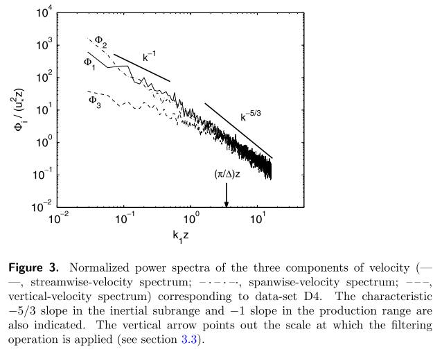
Equation $-\left< \left( \Delta u_1 \right) ^3 \right> +6\nu \frac{d}{dr}\left< \left( \Delta u_1 \right) ^2 \right> =\frac{4}{5}\left< \epsilon \right> r$ is verified only for small scales when the Taylor-microscale Reynolds number $R{\lambda}$ is moderate (Antonia, Chambers & Browne 1983, see also figure 3) ($R{lambda} ≡ u_1^{‘}\lambda/\nu$, where a prime denotes the r.m.s. value and $\lambda ≡ u_1^{‘}/(∂u_1/∂x_1)^{‘}$ is the longitudinal Taylor microscale). At larger scales, the approach to a four-fifths law is expected to be quite slow, as demonstrated by Qian (1999).

Experiment details

On the centreline, the Taylor-microscale Reynolds number $R_{\lambda}$ is about 36, and the Kolmogorov length scale $η$, based on the mean energy dissipation rate $\left<\epsilon\right>_{iso}$, is about 0.5 mm. The measurement location was at 340h from the entrance. The measured mean static pressure gradient and moments of $u_1$ and $u_3$ along the centreline indicated that the flow was fully developed at $x_1 \approx 150h$. Also note that, at the measurement location, the turbulence intensity $u_1^{‘}/U_1$ is about 4% and the ratio $u_1’/u_2’$ about 1.25 on the centreline.

The inclined wires allowed the determination of $u_1$ and $u_3$ fluctuations. The included angle of the two wires is about $100\degree$. The separation between the wires was about 1.2 mm. The hot wires were etched from 2.5 µm diameter Wollaston Pt–10% Rh wires with an active length of about 0.5 mm. The length to diameter ratio of the wires was about 200. The probe was calibrated at the centreline of the channel against a Pitot tube connected to a MKS Baratron pressure transducer (least count = 0.01mm water). The yaw calibration was performed over ±24◦ (using 4◦ steps). For each angle, the probe was relocated at the centreline of the channel. The probe was traversed in the $x_3$-direction between about 1mm from the wall to 2mm beyond the centreline.

The hot wires were operated with constant-temperature anemometers at an overheat ratio of 1.5. The output signals from the anemometers were passed through buck and gain circuits and low-pass filtered (the cut-off frequency fc, which was in the range 400–1250Hz depending on the transverse position of the probe, was set close to the Kolmogorov frequency $U_1/2πη$). The signals were then digitized into a personal computer using a 12 bit A/D converter at a sampling frequency, $f_s$, of 2500 Hz. The record duration was about 60 s. This was estimated to be long enough for the secondand third-order moments of $∆u_1$ and $∆u_3$ to converge.

Estimations of $\left<\epsilon\right>$

$\left<\epsilon\right>$ obtained using different approaches.

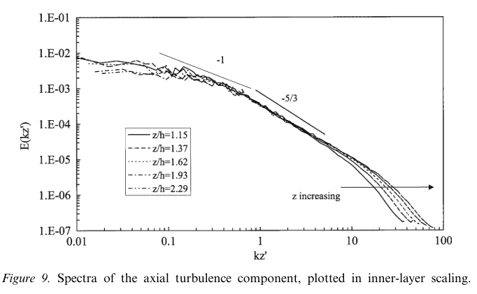
Lawn (1971) inferred $\left<\epsilon\right>$ from the behavior of the $u_1$-spectrum in the IR: \(E(k_1)=K\left<\epsilon\right>^{2/3)}k_1^{-5/3}\) with $K\approx0.51$. The advantage of this approach is that the spectrum needs only to be accurately measured over a medium frequency range, as was noted by Bradshaw (1969). This is essentially the spectral equivalent of Kolmogorov’s equation in the context of determining $\left<\epsilon\right>$. Even if the measurement of $\left<\epsilon\right>$ is in error, the spectral method is robust and more likely to provide meaningful estimates when the Reynolds number is large enough.

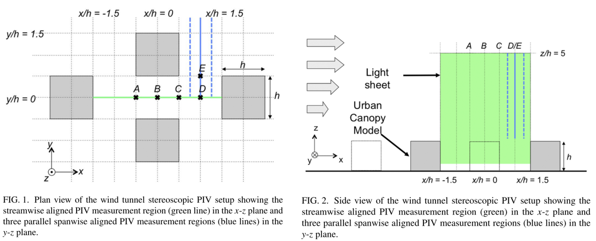
5.(2017)Turbulent kinetic energy budget in the boundary layer developing over an urban-like rough wall using PIV

Karin Blackman; Laurent Perret; Isabelle Calmet; Cédric Rivet

To access the full TKE budget, an estimation of the dissipation (ε) using both the transport equation of the resolved-scale kinetic energy and Large-Eddy (LE) PIV models based on the use of a subgrid-scale model following the methodology used in large-eddy simulations is employed.

(1) Can the TKE budget including dissipation be quantified using PIV measurements in an urban canopy? (2) What is the influence of the presence of the roughness elements on the TKE budget terms? (3) Which coherent structures present in the urban boundary layer are related to the occurrence of backscatter?

Experimental details

The wind tunnel has working section dimensions of 2 m (width) × 2 m (height) × 24 m (length), 5:1 ratio inlet contraction, and a wind speed range of 3–10 $ms^{-1}$.

Within the empty wind tunnel, there is a free-stream turbulence intensity of0.5% with spanwise uniformity to within ±5% (Savory et al., 2013).

To initiate the boundary layer development, five 800 mm vertical tapered spires were used immediately downstream of the contraction followed by a 200 mm solid fence located 750 mm downstream of the spires.

The roughness elements, which consisted of $h = 50$ mm staggered cubes with a plan area packing density $\lambda_p = 25$%.

The experiment was performed with a free-stream velocity $U_{\infty}$= 5.8 $ms^{-1}$ measured with a Pitot-static tube located 15 m downstream of the inlet at the centre of the wind tunnel and $z = 1.5$ m, giving a Reynolds number, based on cube height, of $Re_h = 1.9 × 10^4$.

• Litron double cavity Nd-YAG laser (2 × 200 mJ)
• Two CCD cameras with a 105 mm objective lens
• A frequency of 5 Hz was used between pairs of pulses
• a time-delay of 500 µs was set between two images of the same pair
• The synchronization of the cameras and laser was controlled using Dantec Dynamic Studio software
• perform the PIV analysis of the recorded images by Dantec Dynamic Studio software
• In total 4000 pairs of images were recorded
• 13 min of measurements
• The multi-pass cross-correlation PIV processing resulted in a final interrogation window size of 32 × 32 pixels with an overlap of 50%.
• The PIV measurements had a final spatial resolution of 1.7 mm in the streamwise and 2.2 mm in the vertical directions.

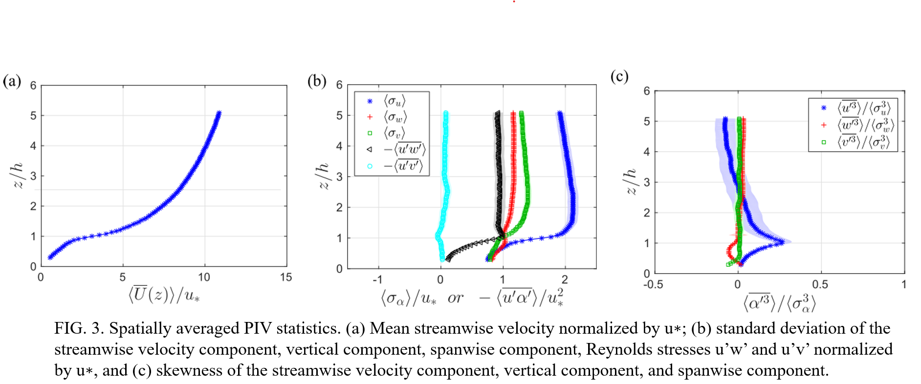
• ==shown in one figure.==

• ==hight order moments calculated by $\left<\alpha^{‘3}\right>/\left<\sigma^{3}\right>$, difference compared with $\left<\alpha^{‘3}/\sigma^{3}\right>$?==

The general form of the TKE budget for a stationary flow is described in equation above, where $Adv$ is advection, $P$ is production, $T$ is turbulent transport, $Ψ$ is pressure transport, $D$ is viscous transport, and $\epsilon$ is dissipation,

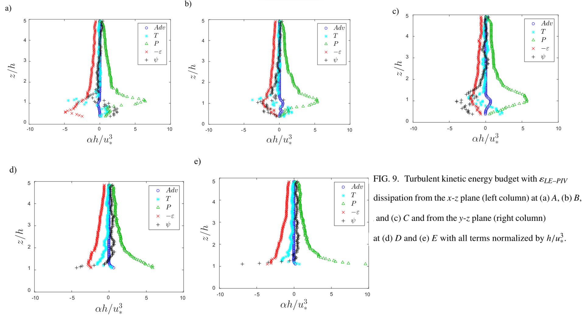
Above the roughness sublayer ($z/h > 2$), the production of energy is balanced by the dissipation, while all other terms are negligible. Close to the obstacles [Fig. 9(a)], the strong shear layer induced by the presence of the roughness elements produces energy. This production term decreases in magnitude with downstream distance as the shear layer develops over the canopy [Fig. 9(c)]. Energy is also dissipated within the shear layer and transported to the canopy and overlying boundary layer through advection, turbulent transport, and pressure transport by the shear layer. Finally, within the canopy, pressure transport is a significant energy sink and is balanced by production and turbulent transport [Figs. 9(b) and 9(c)] except close to the upstream cube where pressure transport becomes an energy source [Fig. 9(a)]. This region, which contains a recirculation region, also exhibits high magnitudes of dissipation and weakly positive production. Away from the shear layer in Figs. 9(d) and 9(e), the production is still balanced by the dissipation; however, the pressure transport becomes weakly positive within the overlying boundary layer suggesting that energy from the shear layer is transported to these regions.

The present work has led to some important findings on the nature of energy production and dissipation in the urban boundary layer. However, the influence of the geometry and packing density (λp) of the roughness used to simulate an urban boundary layer on the TKE budget and sub-grid scale energy transfer remains to be studied. Furthermore, previous work has shown that large-scale coherent structures interact and influence small-scale structures with the shear layer through a non-linear interaction (Blackman and Perret, 2016). Future work will focus on investigating the non-linear energy transfer between these structures.

[1] Castro, I. P., Cheng, H., and Reynolds, R., “Turbulence over urban-type roughness: Deductions from wind-tunnel measurements,” Boundary-Layer Meteorol. 118, 109–131 (2006).

[2] Blackman, K. and Perret, L., “Non-linear interactions in a boundary layer developing over an array of cubes using stochastic estimation,” Phys. Fluids 28, 095108 (2016).

[3] Blackman, K., Perret, L., and Savory, E., “Effect of upstream flow regime on street canyon flow mean turbulence statistics,” Environ. Fluid Mech. 15, 823–849 (2014).

[4] Blackman, K., Perret, L., Savory, E., and Piquet, T., “Wind tunnel modeling of an idealized street canyon flow,” Atmos. Environ. 106, 139–153(2015).

[5] Roth, M., Inagaki, A., Sugawara, H., and Kanda, M., “Small-scale spatial variability ofturbulence statistics, (co)spectra and turbulent kinetic energy measured over a regular array of cube roughness,” Environ. Fluid Mech. 15, 329–348 (2015)

[6] Salizzoni, P., Marro, M., Soulhac, L., Grosjean, N., and Perkins, R. J., “Turbulent transfer between street canyons and the overlying atmospheric boundary layer,” Boundary-Layer Meteorol. 141, 393–414 (2011).

[7] Savory, E., Perret, L., and Rivet, C., “Modelling considerations for examining the meanand unsteady flowin a simple urban-type street canyon,” Meterol. Atmos. Phys. 121, 1–16 (2013).

[8] Takimoto, H., Inagaki, A., Kanda, M., Sato, A., and Michioka, T., “Lengthscale similarity of turbulent organized structures over surfaces with different roughness types,” Boundary-Layer Meteorol. 147, 217–236 (2013).

[9] Takimoto, H., Sato, A., Barlow, J. F., Moriwaki, R., Inagaki, A., Onomura, S., and Kanda, M., “Particle image velocimetry measurements of turbulent flow within outdoor and indoor urban scale models and flushing motions in urban canopy layers,” Boundary-Layer Meteorol. 140, 295–314 (2011).

[10] Zhu, W., van Hout, R., and Katz, J., “On the flow structure and turbulence during sweep and ejection events in a wind-tunnel model canopy,” Boundary-Layer Meteorol. 124, 205–233 (2007).

[11] Castro, I. P., Cheng, H., and Reynolds, R., “Turbulence over urban-type roughness: Deductions from wind-tunnel measurements,” Boundary-Layer Meteorol. 118, 109–131 (2006).

[12] Christen, A., Rotach, M. W., and Vogt, R., “The budget of turbulent kinetic energy in the urban roughness sublayer,” Boundary-Layer Meteorol. 131, 193–222 (2009).

[13] Guala, M., Metzger, M., and McKeon, B. J., “Interactions within the turbulent boundary layer at high Reynolds number,” J. Fluid Mech. 666, 573–604 (2011).

[14] Inagaki, A. and Kanda, M., “Organized structure of active turbulence over an array of cubes within the logarithmic layer of atmospheric flow,” Boundary-Layer Meteorol. 135, 209–228 (2010).

[15] Jimenez, J., “Turbulent flows over rough walls,” Annu. Rev. Fluid Mech. 36, 173–196 (2004).

[16] Marusic, I., McKeon, B. J., Monkewitz, P. A., Nagib, H. M., Smits, A. J., and Screenivasan, K. R., “Wall-bounded turbulent flows at high Reynolds numbers: Recent advances and key issues,” Phys. Fluids 22, 065103 (2010).

[17] Michioka, T. and Sato, A., “Effect ofincoming turbulent structure on pollutant removal from two-dimensional street canyon,” Boundary-Layer Meteorol. 145, 469–484 (2012).

[18] Perret, L. and Savory, E., “Large-scale structures over a single street canyon immersed in an urban-type boundary layer,” Boundary-Layer Meteorol. 148, 111–131 (2013).

[19] Perret, L., Blackman, K., and Savory, E., “Combining wind-tunnel and field measurements ofstreet-canyon flowvia stochastic estimation,” BoundaryLayer Meteorol. 161, 491–517 (2016).

[20] Sheng, J., Meng, H., and Fox, R. O., “A large eddy PIV method for turbulence dissipation rate estimation,” Chem. Eng. Sci. 55, 4423–4434 (2000).

6.(2006)Turbulence over urban-type roughness: deductions from wind-tunnel measurements

IAN P. CASTRO,∗, HONG CHENG and RYAN REYNOLDS

Experiment

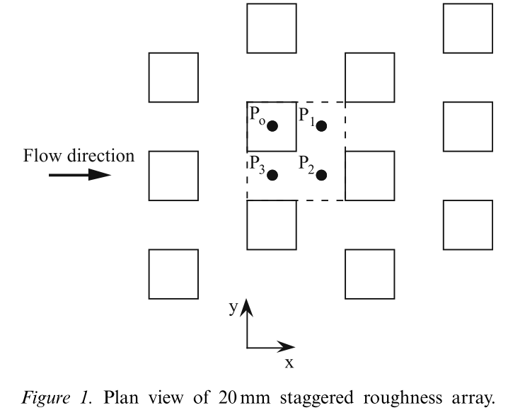
All measurements were carried out around the tunnel (spanwise) centreline, about 3m downstream of the leading edge of the roughness and at a nominal free stream velocity of $10 m s^{−1}$. This gave a boundary-layer thickness of 148mm at the measurement station, a boundary-layer Reynolds number based on momentum thickness of about 12,000, a roughness length, zo, and zero-plane displacement, d, of 1.1 and 17mm, respectively, and a friction velocity, $u_∗/U_o$, of 0.07, where the latter was deduced from form drag measurements obtained by pressure-tapping one of the cubes; alternative ways of obtaining u∗ yielded lower values and gave less satisfactory fits of the mean velocity data to the log-law, as discussed by Cheng and Castro (2002). The streamwise, lateral and vertical coordinates are $(x, y, z)$, with the plane $z=0$​ being the top surface of the baseboard on which the roughness elements were located. Figure 1 shows the roughness arrangement.

The roughness sublayer extends up to $z=1.8h$ and the inertial layer up to $z=2.3h$,as deduced (and discussed) by Cheng and Castro (2002) on the basis of suitably small variations in shear stress.

Profile

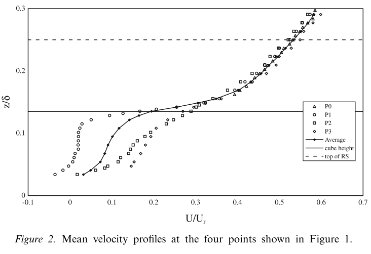
The averaged mean velocity profile shows a strong shear near $z = h$ and contains an inflection point just above that height. This characteristic has prompted the suggestion that the natural instabil-shear near z = h and contains an inflection point just above that height. This characteristic has prompted the suggestion that the natural instabilities near the top of the canopy resemble those in a plane mixing layer rather than a boundary layer (Raupach et al., 1996; Finnigan, 2000).

Single point correlation:

==Obtaining length scales : apply Taylor’s hypothesis to the time scale.==

The autocorrelation coefficient \(R_u(\tau) =\frac{\overline{u(t)u(t+\tau)}}{\overline{u^2}}\) integral time scale \(T_x=\int_{0}^{\infty } R_u(\tau)d\tau\) Taylor’s hypothesis then yields an integral length scale of $L_x =T_xU$​, where U is the local mean velocity.

Two point correlation

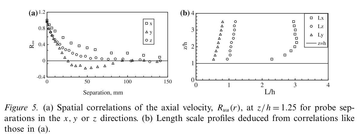
To avoid the shortcomings of applying Taylor’s hypothesis we therefore used two-point measurements to obtain spatial correlations, \(R_{uu}\left( r \right) =\frac{\overline{u\left( r \right) u\left( r+\delta r \right) }}{\sqrt{\overline{u\left( r \right) ^2}}\sqrt{\overline{u\left( r+\delta r \right) ^2}}}\) where $δr$ is the separation of the probes, and thence to deduce the integral length scales $L_x$, $L_y$ and$ L_z$ directly \(L_x=\int_0^{x_c}{R_{uu}\left( x \right) dx}\) with the upper limit of integration determined by the first zero crossing of the correlation coefficient curve.

In these experiments, two single hot-wire probes were used, one of which was fixed at a certain location, and the other traversed vertically, laterally or longitudinally.

A typical set of spatial correlation coefficients with one probe fixed at $z/h=1.25mm$ is shown in Figures 5a and b and shows profiles of the length scales deduced from a complete set of spatial correlation data.

Structure angle

The structure angle, denoting the most likely inclination of the ‘average’ eddy structure (or packet), can be defined as \(\theta =\mathrm{arc}\tan \frac{\varDelta z_m}{\varDelta x}\) where $\Delta x$ is the horizontal probe separation and $\Delta z_m$ is the vertical separation which yields maximum $R_{uu}$. It should be emphasised that these structure angles do not indicate the orientation of individual eddies as they are swept past the measuring point. Rather, they are in some sense an average orientation of all the eddies of different spatial scales and stages of growth and decay and should therefore be interpreted with caution.

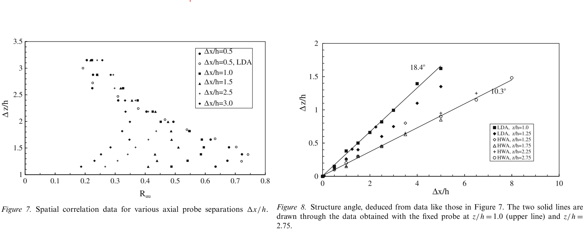
It is clear that as the fixed probe height increased from z/h=1.0 to 2.75, the structure angle decreases from 18.4◦ to 10.3◦, eventually becoming almost constant (about 10◦) for greater reference heights. (Ultimately it must become zero when the fixed probe reaches the free stream). This trend is opposite to the behaviour found in smooth-wall boundary layers (Adrian et al., 2000; Marusic, 2001) where the structure angle increased monotonically with increasing distance from the wall, from a minimum nearest the wall of about 10◦ (although by z/δ =0.1 the latter had increased to 20◦).

The ==inertial sublayer covered the range $1.85 <z/h< 2.3$== (Cheng and Castro, 2002) and a clear correlation peak was detected even with the traversing probe well above this log-law region, so our data support the idea that coherent turbulence structures appear not only in the near-wall region and logarithmic regions but also well into the middle of the boundary layer, as reported by Adrian et al. (2000). These organised structures may be the main eddies associated with near wall transport processes and thus would have an important role in effecting pollutant dispersion over urban roughness. However, this is not yet proven and it is at least possible that the small-scale structures near z=h, discussed in the previous section, will be crucial in contributing to transport of scalar quantities across the strong shear region between the lower canopy flow and the upper part of the roughness sublayer.

The turbulent kinetic energy (TKE) budget illustrates the relative importance of the physical processes that govern the turbulent flow. For stationary flow with no buoyancy forces under neutral conditions, the TKE balance can be simplified as:

\(\frac{Dk}{Dt}=-\overline{uw}\frac{\partial U}{\partial z}+\left( \overline{w^2}-\overline{u^2} \right) \frac{\partial U}{\partial x}-\frac{1}{\rho}\frac{\partial \overline{wp}}{\partial z}-\frac{\partial \overline{wk}}{\partial z}-\epsilon\) ​ $A$ $P_{ss}$ $P_{sn}$ $T_p$ $T_t$ $D$

where $2k≡q^2=(u^2+v^2+w^2)$, $\overline{wk}=(\overline{u^2w}+\overline{v^2w}+\overline{w^3})/2$ and we assume that $\overline{v^2w}=(\overline{u^2w}+\overline{w^3})/2$. In the above equation, $A$, $P_{ss}$, $P_{sn}$, $T_p$, $T_t $ and $D$ are the advection, shear production, normal stress production, pressure transport, turbulent transport and dissipation terms, respectively.

$A$, $P_{ss}$, $P_{sn}$, $T_p$, $T_t $ can be calculated directly from the measurements and $D$​ can be estimated from power spectral density measurements, with an error of perhaps 20% at most.

$k$ here is the wavenumber defined by $k =2πf/U$ and $z’ =z−d$.

==$T_p$​ can be inferred indirectly as a residual after determination of all other terms from the experimental data.==

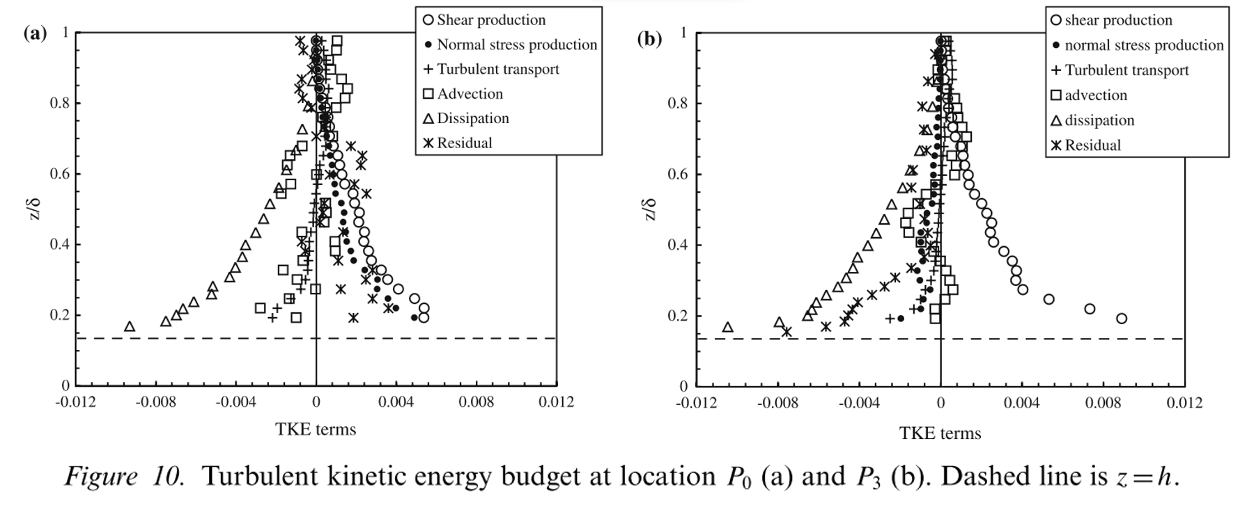
Figure 10 shows the resulting balances for P0 and P3; all terms have been normalized by ($U^3_r /δ$). Note first that the significance of the normal stress production term is quite different at the two locations. It is almost as large as shear production in the roughness sublayer at $P_0$ (Figure 10a). This is perhaps not surprising since the flow is spatially much more inhomogeneous than in a regular boundary layer and this inhomogeneity may well be largest (e.g. longitudinal gradients are largest) immediately over a cube, where the shear layers separating from the leading edges are developing most rapidly. Secondly, observe that the residual term is consistently large and negative at $P_3$. This suggests that pressure transport is relatively significant, although it is possible that the errors in the measured terms contribute significantly to this residual. Certainly, at $P_0$, the residual is rather more scattered, but it is consistently of opposite sign to that at $P_3$​, representing a source of energy rather a sink. As expected, shear production is approximately balanced by the dissipation in the surface layer at both locations and the turbulent transport term is a measurable energy sink there.

Conclusions

analysing single- and two-point velocity statistics obtained in flow over urban roughness in a wind tunnel

Examination of the turbulent kinetic energy budget indicates that shear production is a principle source of energy in the region above the canopy, as expected, and that turbulent transport plays an important role in the surface layer.

Around the top of the canopy region there is some evidence of two-scale behavior,

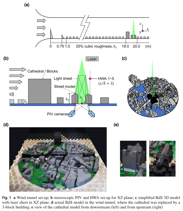
7.(2024)Effect of urban morphology and an upstream tall building on the scale interaction between the overlying boundary layer and a street canyon

Haoran Du · Laurent Perret · Eric Savory

The interaction of large- and small-scale velocity fluctuations between a street canyon flow and the overlying boundary layer, under the influence of a local morphological model and a single upstream tall building, is investigated.

Understanding the dynamic transport of air and pollutants across the shear layers of street buildings to the overlying atmospheric boundary layer is crucial to the enhancement of urban air quality.

In the case of both a large enough ratio of boundary layer thickness to roughness $δ/h_1$​ and a δ+ = δu∗/ν), the inertial layer (or the log-layer) of an urban-type rough-wall boundary layer has qualitatively similar dynamical and structural properties as smooth-wall turbulent boundary layer flows (Volino et al. 2007; Takimoto et al. 2013;Perretetal. 2019), containing coherent structures such as Large-Scale Motions (LSMs), which are packets of hairpin vortices (Zhou et al. 1999;Adrianetal. 2000), and Very Large-Scale Motions (VLSMs) (Marusic et al. 2010b), which are elongated, low- and high-momentum regions meandering horizontally above the wall.

1. How does the morphology impact the scale interaction in the overlying boundary layer and the street canyon, in comparison with the homogeneous roughness model?
2. What is the impact of a single upstream tall building and its height on the scale interaction in the boundary layer and the street canyon?
3. Will an irregularly-shaped upstream tall building affect the scale interaction, in comparison with an idealized regular, symmetric building?

Experiment

• Wind tunnel: This open-loop wind tunnel has test section dimensions of 24m (length) × 2m (width) × 2m (height) and a 5:1 ratio inlet contraction.
• five vertically tapered spires measuring 800mm in height and 134mm in base width were positioned at the beginning of the test section, after which a solid fence measuring 200mm in height and then a 17m fetch of staggered cubes of height $h1 = 50 mm$ and plan area density $λp1= 25%$ were placed across the test section to fully develop the boundary layer flow.
• A1:200 scalemorphographicmodel
• A Dantec stereoscopic particle image velocimetry (S-PIV) system was used to measure the 3-component velocity fields
• A Litron double cavity NdYAG laser (2 × 200 mJ), light sheet in the XZ plane.
• Olive oil droplets of 1 µm average diameter generated by a LaVision Laskin-Nozzle aerosol generator
• Two 2048 × 2048 CCD cameras with 105mm objective lenses were installed under the wind tunnel floor on each side of the light sheet and angled at 45◦ towards the sheet.
• 10,000 pairs of images were recorded at a frequency of 7.4 Hz, with a time delay of 300 µs between two images of the same pair.
• The final spatial resolution for the experiments was 1.6 mm (0.022 Wc) and 3.2 mm (0.028 h2) in the streamwise (x) and vertical directions (z), respectively.
• final interrogation window size of 32 × 32 pixels with an overlap of 50%.
• Five single hot-wire anemometer (HWA) probes with a sampling frequency of 15 kHz, were evenly placed in the lateral direction with a spacing of 50mm (0.25 Wb)at z/h = 3 over the centre of the downstream street canyon building. ==The HWA measurements were performed synchronously with the PIV measurements.==

POD-LSE

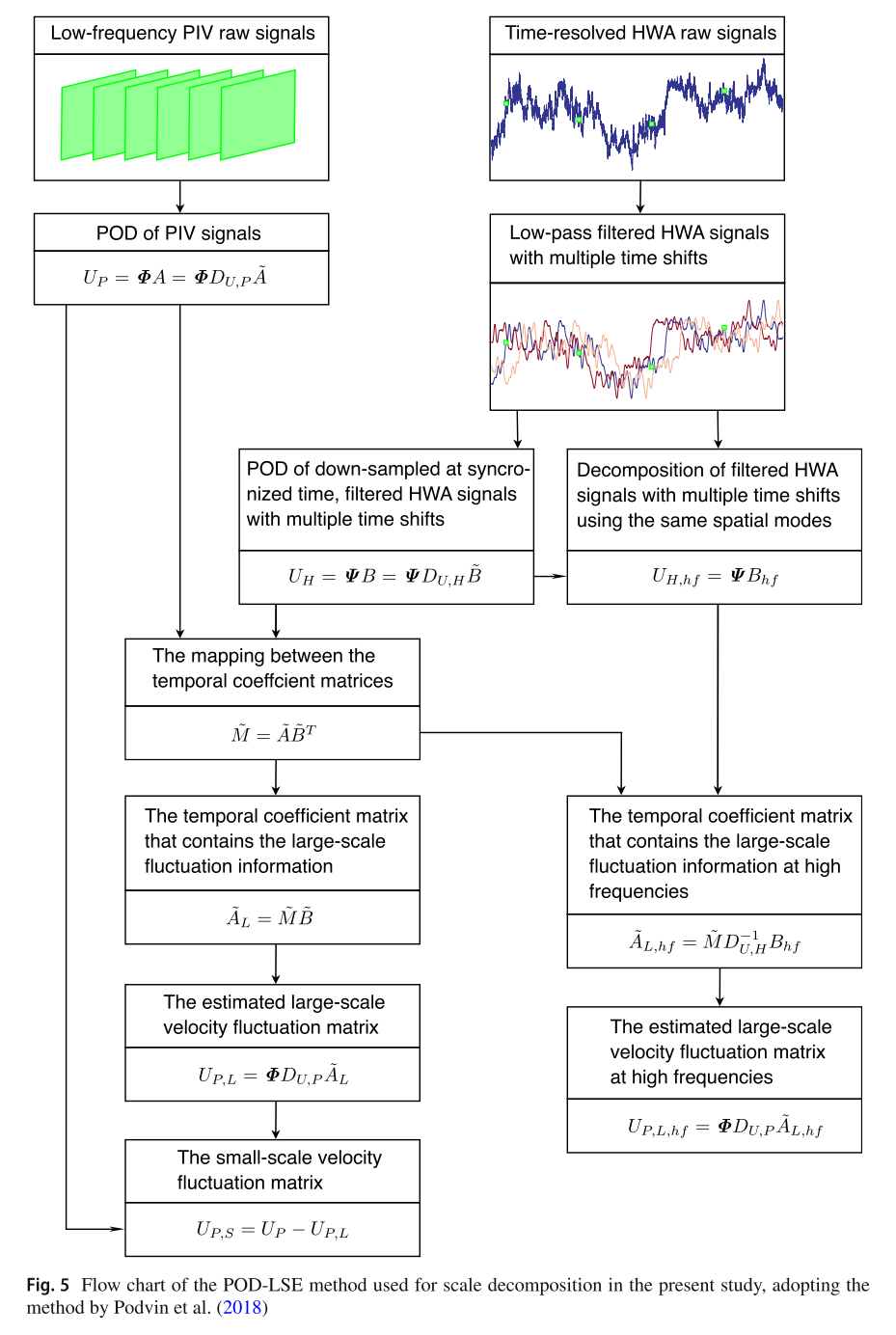
The streamwise length scales of the large-scale streamwise velocity fluctuations are estimated using the temporal auto-correlation $R_{u_Lu_L}$​ and Taylor’s hypothesis of frozen turbulence, \(L_{u_L}\left( z \right) =\overline{U}\left( z \right) \int_0^{\infty}{R_{u_Lu_L}\left( z, \tau \right)}d\tau\)

Skewness Decomposition²

[2]Blackman K, Perret L, Savory E (2018) Effects of the upstream flow regime and canyon aspect ratio on non-linear interactions between a street-canyon flow and the overlying boundary layer. Boundary-Layer Meteorol 169:537–558 \(u'=u_L'+u_S' \\ u'^3=\left( u_L'+u_S' \right) ^3 \\ u'^3=u_L'^3+3u_L'^2u_S'+3u_L'u_S'^2+u_S'^3\)

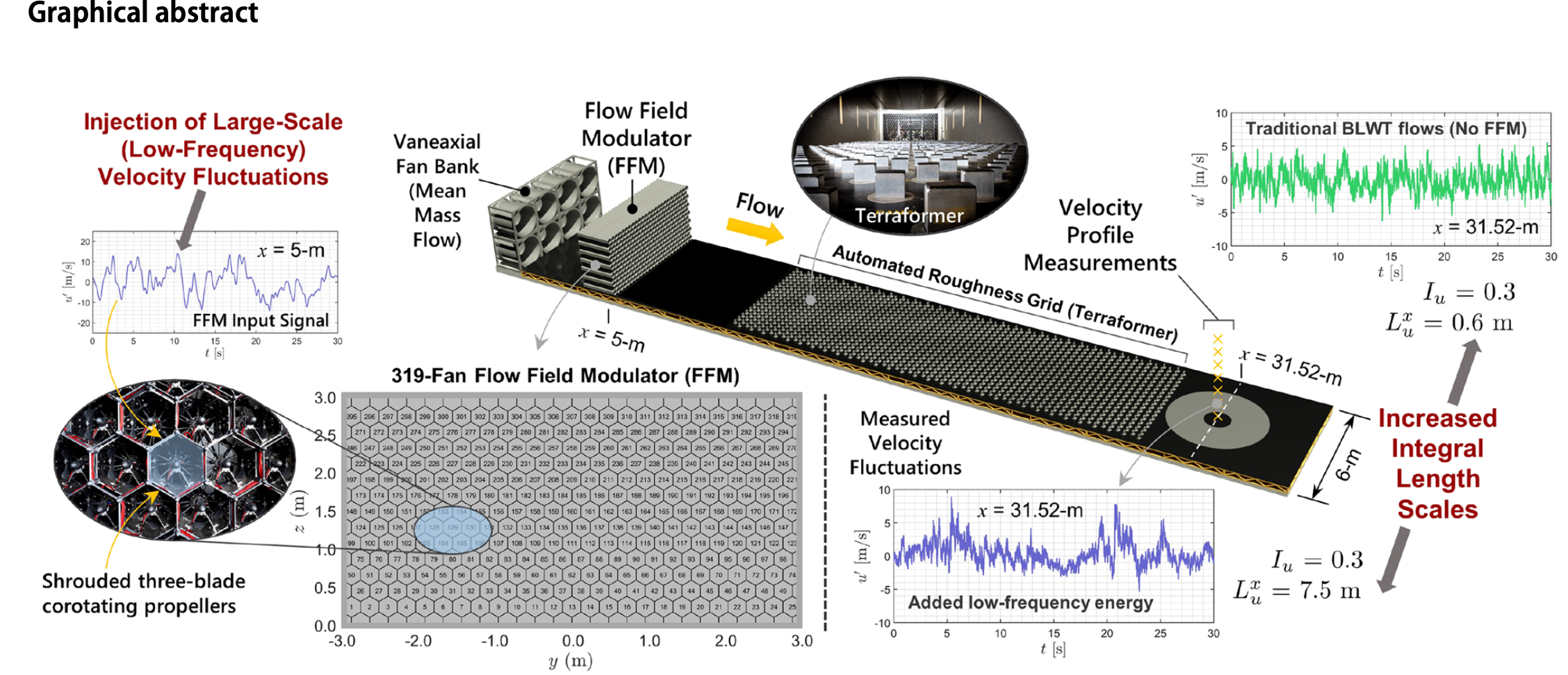
8.(2024)Automated large‐scale and terrain‐induced turbulence modulation of atmospheric surface layer flows in a large wind tunnel

Nasreldin O. Mokhtar · Pedro L. Fernández‐Cabán1 · Ryan A. Catarelli

9.Secondary motions and wall-attached structures in a turbulent flow over a random rough surface

10.（2018）Effects of the Upstream-Flow Regime and Canyon Aspect Ratio on Non-linear Interactions Between a Street-Canyon Flow and the Overlying Boundary Layer

Karin Blackman1 · Laurent Perret1,2 · Eric Savory3

Useful expressions: RSL, ISL, scale interaction

1.==The flow associated with street canyons that form the urban-canopy roughness comprises several regions, including the roughness sublayer, whose depth depends on the density and height of the roughness elements, and the inertial layer, which contains large-scale structures influenced by the surface characteristics (Rotach et al. 2005). Within these regions, the flow comprises complex coherent structures that have been identified through direct numerical simulation (DNS) (Coceal et al. 2007; Lee et al. 2011, 2012), wind-tunnel experiments (Castro et al. 2006; Takimoto et al. 2013) and field experiments (Inagaki and Kanda 2008, 2010).==

2.==These coherent structures consist of large-scale turbulent organized motions of either high or low momentum that form well above the roughness in the inertial layer, shear layers that form within the roughness sublayer along the top ofthe upstream roughness elements and contain small-scale structures induced by the presence of the roughness, and a recirculation region within the street canyon (Coceal et al. 2007).==

3.==These structures, especially how they interact with one another, are ofparticular interest since they govern the intermittent turbulent events, such as ejections (Q2: u < 0and w > 0) and sweeps (Q4: u > 0and w < 0), that produce the transport of heat, momentum and pollution between the street canyon and the overlying roughness sublayer and inertial layer (Takimoto et al. 2011; Perret and Savory 2013).==

4.==The present study focuses on the roughness sublayer and lowest region of the inertial sublayer, since this is the region in which scale interactions important to the ventilation of street canyons are expected to occur.==

Target:

1. What is the quantitative influence of the roughness configuration on the non-linear relationship between large-scale structures in the inertial layer and small-scale structures induced by the presence of the roughness in the roughness sublayer?

2. What is the quantitative influence of the street-canyon aspect ratio on this non-linear relationship?

Experiment:

wind tunnel: $2m(W)\times 2m(H) \times 24m(L)$​. The freestream turbulence intensity within the empty wind tunnel of $0.5$% with spanwise uniformity to within $\pm 5$%.

Five 800-mm vertical tapered spires were used immediately downstream of the contraction to initiate the boundary-layer development and were followed by a $200$-mm high solid fence located $750$ mm downstream of the spires. An initial $13$-m fetch of $50$-mm staggered cubic roughness elements with a plan area density of $\lambda_p=25$ % was used to further develop the boundary layer. The roughness elements over the remaining portion of the wind tunnel were either 50-mm cubes (arranged in a staggered array with $\lambda_p=25$ % ) or 50-mm square-section, 2D bars that spanned the width of the tunnel, with an element spacing of either 1h ($\lambda_p=25$ % ) or 3h ($\lambda_p=25$ % ). These configurations result in a $1\colon200$​ scaling of a suburban-type atmospheric boundary layer (Blackman et al. 2015).

Boundary-Layer Characteristics:

The logarithmic-law parameters, aerodynamic roughness length ($z_0$) and displacement height ($d$), were determined by fitting the vertical profile of the streamwise velocity component to the logarithmic law (Blackman et al. 2015) while the friction velocity, $u_\ast$, was estimated from the vertical profile of the Reynolds shear stress in the constant-stress region located just above the roughness elements. ==Within the wind tunnel a region of constant stress is not typically observed so the shear stress must be approximated by an average of the shear stress over a region, selected based on a combination of the flattest region of the profile and the expected value for the configuration from the literature.==

Although we recognize that this method of estimating $u_\ast$​ does not normally yield accurate results in rough-wall boundary layers the conclusions are unlikely to be affected. For further details, see Blackman³.

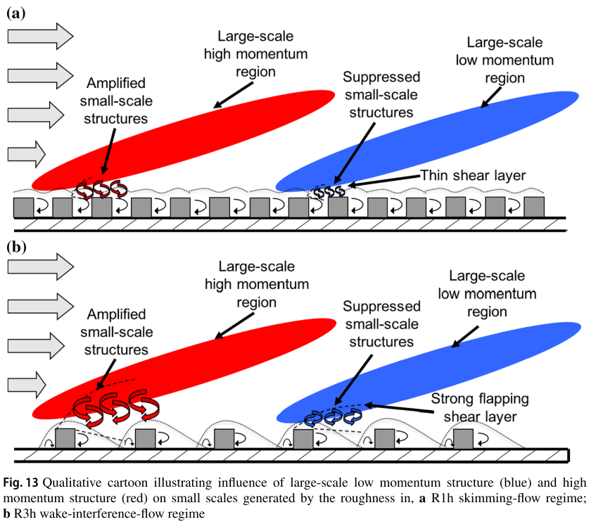
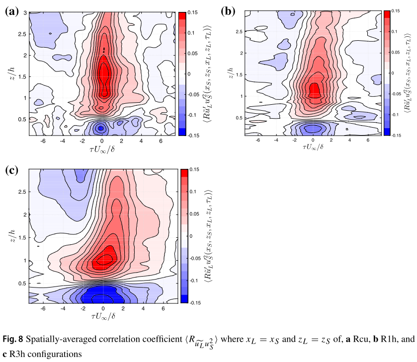
The skimming-flow regime (R1h) is shown to increase $\overline{u}$ , $\sigma_u$, $\sigma_w$ and $\sigma_v$, while $\overline{u’w’}$ decreases compared to the wake-interference regime (R3h). The 3D roughness (Rcu) falls between the skimming-flow and wake-interference-flow regimes except in the case of $\sigma_w$ and $\sigma_v$​​, which are similar to wake-interference profiles.

Stochastic Estimation Model⁴²

In the stochastic estimation method the approximated near-wall large-scale fluctuating velocity ($\widetilde{u^{\prime NW}}$) is calculated at each location of interest from coefficients ($A_{l}^{n}$) and a reference velocity signal ($u_{L}^{\prime BL}$​​​).

The LSE coefficients ($A_{l}^{n}$ ) are determined from the cross-correlation of the low-pass filtered large-scale fluctuations and the raw near-wall PIV signal at the location in space (x, y, z) that is to be predicted, as well as the autocorrelation of the large-scale signal,

A time lag $\Delta t=0.2$ s with a maximum delay of t −1 s to 1 s is introduced to these correlations to preserve the time separation of the conditional and unconditional events so that each coefficient represents the correlation between events at a specific instance in time. $N_{ref}$ is the number of reference locations and $2N_t + 1$​ is the number of time lags used.

Conceptual figure:

Inspiration:

1. Calculate the $R_{\widetilde{u}{L}u{S}^{2}}$, \(R_{\widetilde{u}_{L}u_{S}^{2}}(x_{S},z_{S},x_{L},z_{L},\tau_{L})=\frac{\widetilde{u_{L}^{\prime}}(x_{L},z_{L},t+\tau_{L})u_{S}^{\prime2}(x_{S},z_{S},t)}{\sqrt{\widetilde{u_{L}^{\prime}}^{2}(x_{L},z_{L})}\sqrt{u_{S}^{\prime2}(x_{S},z_{S})}^{2}}\)

1. Calculate the inclined angle from the hot-wire data by Taylor hypothesis.

2. The introduction, excellent.

11.(2016)Non-linear interactions in a boundary layer developing over an array of cubes using stochastic estimation

Karin Blackman1,a) and Laurent Perret1,2

In the present work, a boundary layer developing over a rough-wall consisting of staggered cubes with a plan area packing density, $\lambda_p$ = $25$%, is studied within a wind tunnel using combined particle image velocimetry and hot-wire anemometry to investigate the non-linear interactions between large-scale momentum regions and small-scale structures induced by the presence of the roughness.

Analysis of the scale-decomposed skewness of the turbulent velocity ($u’$) shows a significant contribution of the non-linear term $\overline{u^{\prime}_Lu_S’^{2}}$ , which represents the influence of the large-scales ($u’_L$) onto the small-scales ($u’_S$). It is shown that this non-linear influence of the large-scale momentum regions occurs with all three components of velocity in a similar manner.

==The depth of the roughness sub-layer depends on the density and height of the roughness elements and is followed by the inertial layer where the turbulence contains large-scale structures that are influenced by the surface characteristics==

==Within these regions the flow is comprised of complex coherent structures that have been identified through Direct Numerical Simulation (DNS)==

==These coherent structures consist of==

==(1) large-scale turbulent organized structures of either high or low momentum that form well above the roughness in the inertial layer from groups of hairpin vortices;==

==(2) shear layers that form within the roughness sub-layer along the top of the upstream roughness elements and contain small-scale structures induced by the presence of the roughness;==

==(3) a recirculation region within the canopy layer (Fig. 1)==

Several methods have been used to identify and separate large-scale fluctuations within the rough-wall boundary layer such as Proper Orthogonal Decomposition (POD) (Perret and Rivet, 2013), wavelength spectral filtering (Nadeem et al., 2015), and spatial filtering

12.(2017)Self-similarity of wall-attached turbulence in boundary layers

Woutijn J. Baars1,†, Nicholas Hutchins1 and Ivan Marusic1

spectral coherence analysis

‘self-similar’ will refer to the feature of geometrical self-similarity of various-sized turbulent motions. ‘Wall-attached’ will refer to the energy portions of turbulent fluctuations in the outer region, which are coherent with the wall-shear stress signature or the velocity fluctuations at a reference position deep within the near-wall region.

References